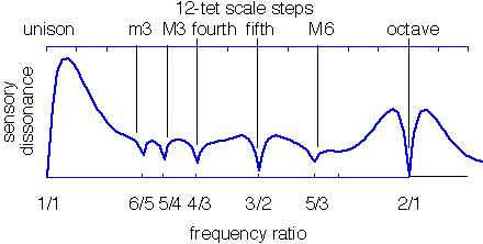
|
""" |
|
Python translation of http://sethares.engr.wisc.edu/comprog.html |
|
""" |
|
import numpy as np |
|
|
|
|
|
def dissmeasure(fvec, amp, model='min'): |
|
""" |
|
Given a list of partials in fvec, with amplitudes in amp, this routine |
|
calculates the dissonance by summing the roughness of every sine pair |
|
based on a model of Plomp-Levelt's roughness curve. |
|
|
|
The older model (model='product') was based on the product of the two |
|
amplitudes, but the newer model (model='min') is based on the minimum |
|
of the two amplitudes, since this matches the beat frequency amplitude. |
|
""" |
|
# Sort by frequency |
|
sort_idx = np.argsort(fvec) |
|
am_sorted = np.asarray(amp)[sort_idx] |
|
fr_sorted = np.asarray(fvec)[sort_idx] |
|
|
|
# Used to stretch dissonance curve for different freqs: |
|
Dstar = 0.24 # Point of maximum dissonance |
|
S1 = 0.0207 |
|
S2 = 18.96 |
|
|
|
C1 = 5 |
|
C2 = -5 |
|
|
|
# Plomp-Levelt roughness curve: |
|
A1 = -3.51 |
|
A2 = -5.75 |
|
|
|
# Generate all combinations of frequency components |
|
idx = np.transpose(np.triu_indices(len(fr_sorted), 1)) |
|
fr_pairs = fr_sorted[idx] |
|
am_pairs = am_sorted[idx] |
|
|
|
Fmin = fr_pairs[:, 0] |
|
S = Dstar / (S1 * Fmin + S2) |
|
Fdif = fr_pairs[:, 1] - fr_pairs[:, 0] |
|
|
|
if model == 'min': |
|
a = np.amin(am_pairs, axis=1) |
|
elif model == 'product': |
|
a = np.prod(am_pairs, axis=1) # Older model |
|
else: |
|
raise ValueError('model should be "min" or "product"') |
|
SFdif = S * Fdif |
|
D = np.sum(a * (C1 * np.exp(A1 * SFdif) + C2 * np.exp(A2 * SFdif))) |
|
|
|
return D |
|
|
|
|
|
if __name__ == '__main__': |
|
from numpy import array, linspace, empty, concatenate |
|
import matplotlib.pyplot as plt |
|
|
|
""" |
|
Reproduce Sethares Figure 3 |
|
http://sethares.engr.wisc.edu/consemi.html#anchor15619672 |
|
""" |
|
freq = 500 * array([1, 2, 3, 4, 5, 6]) |
|
amp = 0.88**array([0, 1, 2, 3, 4, 5]) |
|
r_low = 1 |
|
alpharange = 2.3 |
|
method = 'product' |
|
|
|
# # Davide Verotta Figure 4 example |
|
# freq = 261.63 * array([1, 2, 3, 4, 5, 6]) |
|
# amp = 1 / array([1, 2, 3, 4, 5, 6]) |
|
# r_low = 1 |
|
# alpharange = 2.0 |
|
# method = 'product' |
|
|
|
n = 3000 |
|
diss = empty(n) |
|
a = concatenate((amp, amp)) |
|
for i, alpha in enumerate(linspace(r_low, alpharange, n)): |
|
f = concatenate((freq, alpha*freq)) |
|
d = dissmeasure(f, a, method) |
|
diss[i] = d |
|
|
|
plt.figure(figsize=(7, 3)) |
|
plt.plot(linspace(r_low, alpharange, len(diss)), diss) |
|
plt.xscale('log') |
|
plt.xlim(r_low, alpharange) |
|
|
|
plt.xlabel('frequency ratio') |
|
plt.ylabel('sensory dissonance') |
|
|
|
intervals = [(1, 1), (6, 5), (5, 4), (4, 3), (3, 2), (5, 3), (2, 1)] |
|
|
|
for n, d in intervals: |
|
plt.axvline(n/d, color='silver') |
|
|
|
plt.yticks([]) |
|
plt.minorticks_off() |
|
plt.xticks([n/d for n, d in intervals], |
|
['{}/{}'.format(n, d) for n, d in intervals]) |
|
plt.tight_layout() |
|
plt.show() |


Well, here is a scale consisting of intervals 1, 36/25, 25/16, 16/9, 9/4, 25/9 (the most significant intervals picked out by the dissonance curve, above, in order). It's a bit wrong to call these all "hydrogen," since we'd have to vary the mass or coupling strength to get anything but the lowest tone, and that one has been shifted many octaves into human hearing. It's like we had a musical instrument consisting of many onia, such as muonium and positronium, each with a mass scaled to be in harmony with the others, where harmony is defined by the squares of small integer ratios.
https://gist.github.com/jpivarski/5e4908b09f4f9a244496d4d214e5c769/raw/c43bfaec1927400f0ec39acf0f592ca82d2927ff/hydrogen-scale.wav
Since the amplitudes matter a lot in determining the sound, I found a realistic table of transition probabilities (see my script): what we're hearing is the sound of photons released from atoms that are completely saturated with energy when "plucked." (I think a guitar string would do the same.) Each tone is rough just by itself because this spectrum includes many nearly equal frequencies ("fine splittings"). I didn't take that into consideration when making the dissonance curve. It wouldn't change the locations of the consonant dips, but it would make all of them a lot less consonant.
Maybe I should do one with a less realistic spectrum, so that we can try to hear how the tones of this scale are actually more consonant with each other than randomly chosen ones? (This was already a rabbithole!)